


This guide is part of the Microsoft Excel 2013 series
1.
Add a print button to the tool bar in excel 2013
2. How to add a background image in excel 2013
3. How to add a button to the tool bar in excel 2013
4. How to add a column to a spreadsheet in excel 2013
5. How to auto fit column width in excel 2013
6. How to convert a column into a row in excel 2013
7. How to create a drop down menu in excel 2013
8. How to create a pie chart in excel 2013
9. How to create a pivot table in excel 2013
10. How to create a popup window in excel 2013
Make: Microsoft
Model / Product: Excel
Version: 2013
Objective / Info: Learn To Create A Pivot Table In Excel 2013.
Model / Product: Excel
Version: 2013
Objective / Info: Learn To Create A Pivot Table In Excel 2013.
1
Launch Excel by clicking on the desktop icon.
2
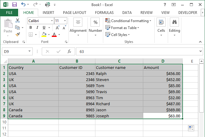
First of all, fill the Excel Worksheet with the relevant data. Now, select the entire data range you wish to create a pivot table for.
3
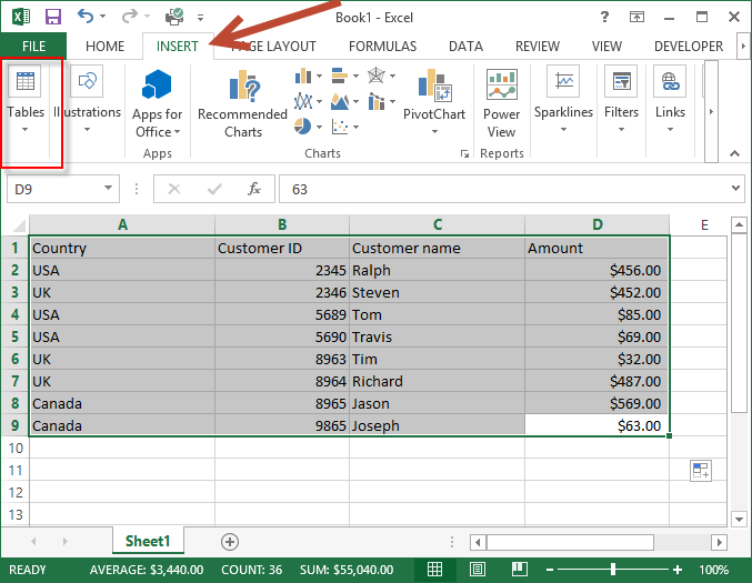
Go to the ‘Insert’ tab and click the ‘Pivot Table’ icon to insert the Pivot Table.
4
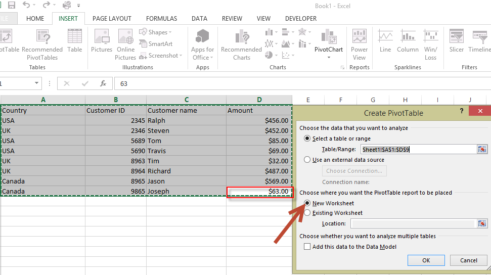
Select the targeted cell you wish the Pivot Table to be inserted in. For beginners, select ‘New Worksheet’ option to create the new worksheet with the Pivot Table.
5
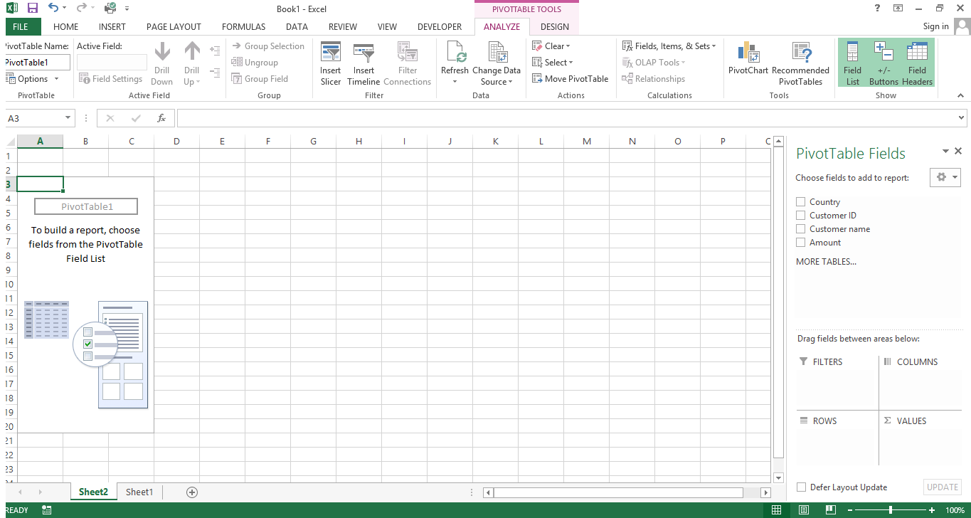
The new worksheet will open. On the right, you can see the Pivot Table Panel containing useful options for working with the table.
6
This task should be complete. Review the steps if you had any issues and try again.Submit questions or request for more guides in the questions section below.comments powered by Disqus
 Ask a question or provide an answer