


This guide is part of the Microsoft Excel 2013 series
1.
Add a print button to the tool bar in excel 2013
2. How to add a background image in excel 2013
3. How to add a button to the tool bar in excel 2013
4. How to add a column to a spreadsheet in excel 2013
5. How to auto fit column width in excel 2013
6. How to convert a column into a row in excel 2013
7. How to create a drop down menu in excel 2013
8. How to create a pie chart in excel 2013
9. How to create a pivot table in excel 2013
10. How to create a popup window in excel 2013
Make: Microsoft
Model / Product: Excel
Version: 2013
Objective / Info: Learn how to create a drop down menu in excel 2013.
Model / Product: Excel
Version: 2013
Objective / Info: Learn how to create a drop down menu in excel 2013.
1
Open Excel by double left clicking the icon on the desktop or start menu or open the document that you want to work on.
2
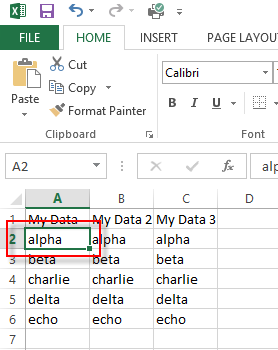
Click on the cell where you want to place the drop down menu. Note :
In this example, we are going to keep cell A1 and use the data in cells A2-A6 as drop down options so we select A2.
3
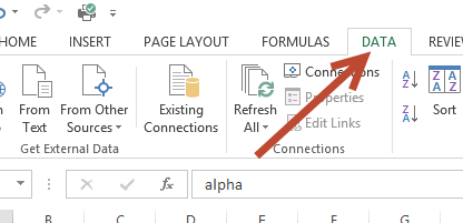
Select the "Data" tab from the menu bar.
4
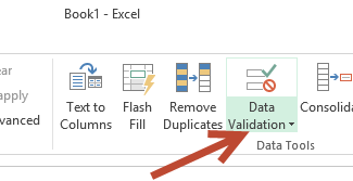
Click the "Data Validation" button.
5
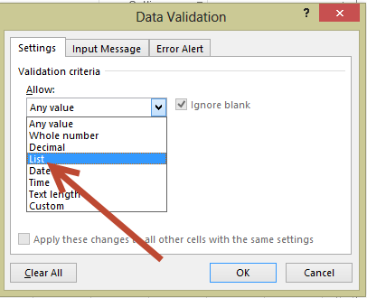
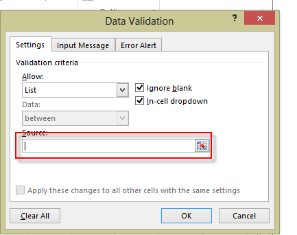
Select "List" from the "Allow" drop down field.
6
Left click on the "Source" field.
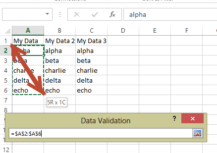
7
Click and drag across the cells that you want to include in your drop down list.
Note :
The source fields are the cells that contain the options that you want to appear in your drop down list. These cells can be located anywhere in your worksheet or workbook.
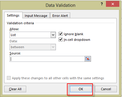
8
Click the "Ok" button when you are finished making your selection.
9
At this point you can click the cell and you should see a drop down list containing the data you selected.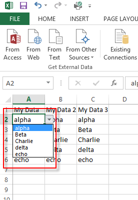
10
This task should be complete. Review the steps if you had any issues and try again.Submit questions or request for more guides in the questions section below.comments powered by Disqus
 Ask a question or provide an answer