


This guide is part of the Microsoft Excel 2013 series
1.
Add a print button to the tool bar in excel 2013
2. How to add a background image in excel 2013
3. How to add a button to the tool bar in excel 2013
4. How to add a column to a spreadsheet in excel 2013
5. How to auto fit column width in excel 2013
6. How to convert a column into a row in excel 2013
7. How to create a drop down menu in excel 2013
8. How to create a pie chart in excel 2013
9. How to create a pivot table in excel 2013
10. How to create a popup window in excel 2013
Make: Microsoft
Model / Product: Excel
Version: 2013
Objective / Info: Learn to create a pie chart in excel 2013.
Model / Product: Excel
Version: 2013
Objective / Info: Learn to create a pie chart in excel 2013.
1
Open Excel by clicking the icon on your desktop or start menu.
2
You should see a blank new sheet.
3
Populate the data into the cells as pictured.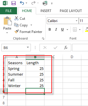
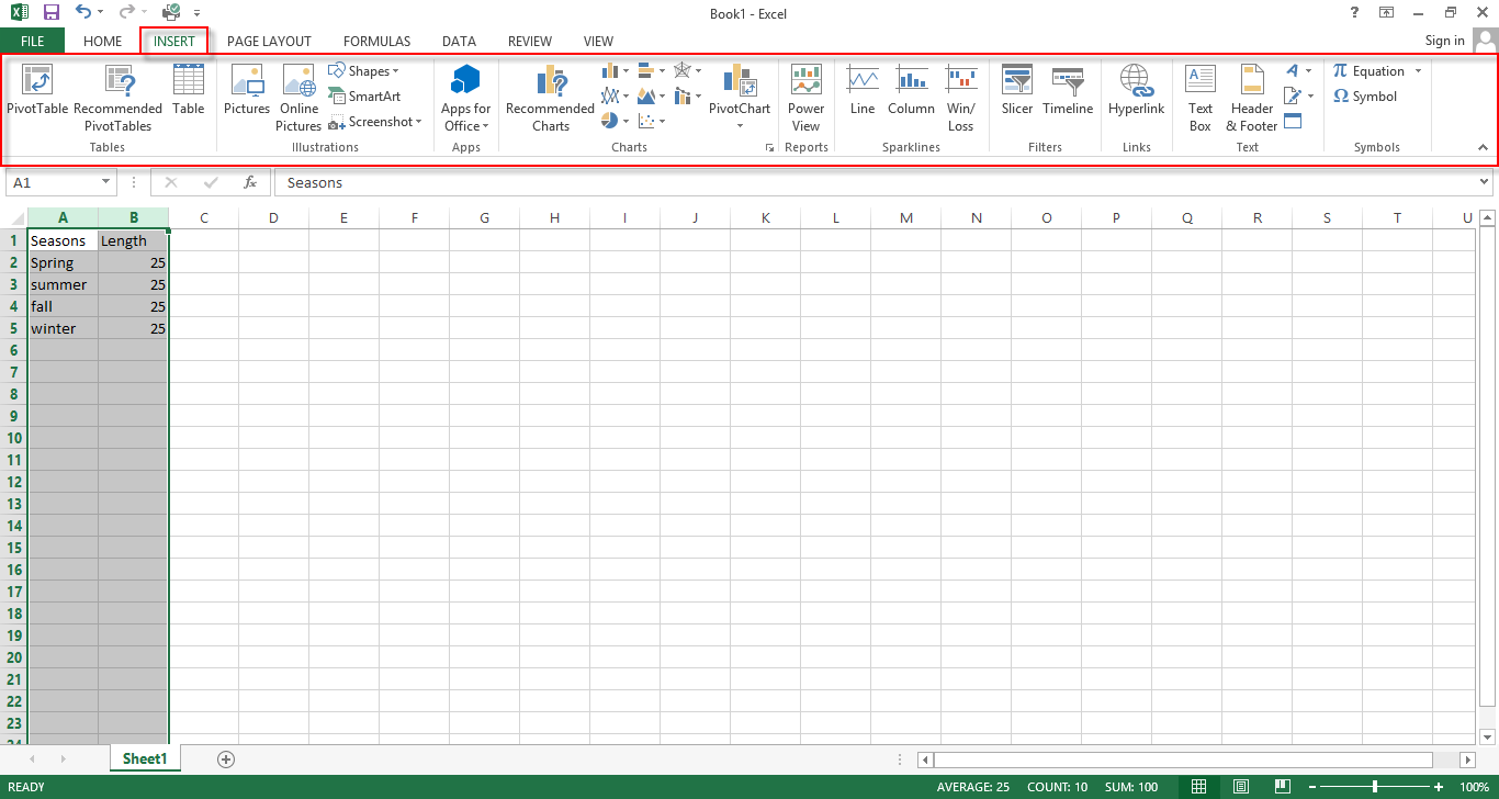
4
Select the spreadsheet data that will be contained in the chart. You select by pressing the left click button on the mouse while over cell "A1" and holding it while you drag it across the data you want to select. After all of your data is selected, release the left mouse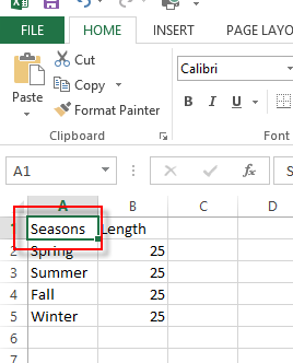
5
While the data is selected, left click on the "Insert" link on the menu. A new set of menu options should appear.
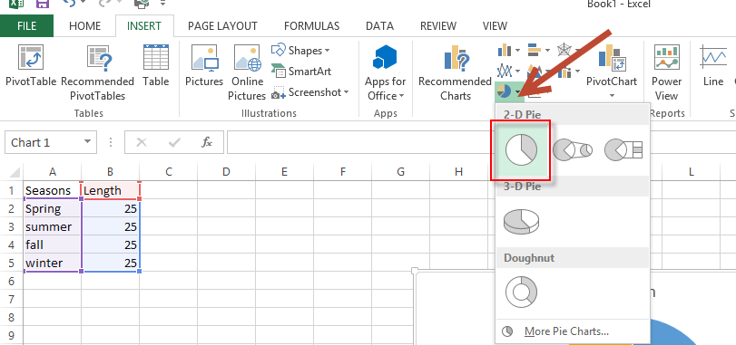
6
Select the “Pie” button and then click the pie chart of your choice
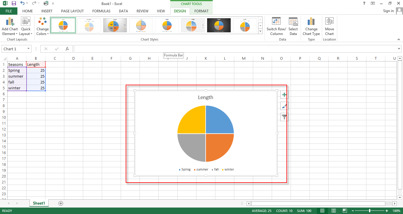
7
The pie chart should be inserted into your spreadsheet somewhere near or in the center of the page.
8
Make any further edits to the chart or the data in the cells and save your pie chart by clicking "File".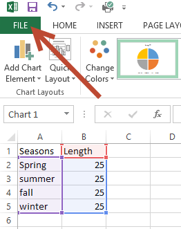
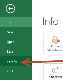
9
Click "Save As" and move the file to a location of your choice. Note :
You can also click "Save" if you have previously saved the file.
10
This task should be complete. Review the steps if you had any issues and try again.Submit questions or request for more guides in the questions section below.comments powered by Disqus
 Ask a question or provide an answer