


This guide is part of the Microsoft Excel 2019 series
1.
How to add a background image in Excel 2019
2. How to add a column to a spreadsheet in Excel 2019
3. How to add a printer to the toolbar in Excel 2019
4. How to add a URL to a spreadsheet in Excel 2019
5. How to auto fit column width in Excel 2019
6. How to change the colors of tabs in Excel 2019
7. How to convert a column into a row in Excel 2019
8. How to copy a worksheet in Excel 2019
9. How to create a drop down menu in Excel 2019
10. How to create a pie chart in Excel 2019
Make: Microsoft
Model / Product: Excel
Version: 2019
Objective / Info: Learn how to create a pie chart in the 2019 version of Microsoft Excel.
Model / Product: Excel
Version: 2019
Objective / Info: Learn how to create a pie chart in the 2019 version of Microsoft Excel.
1
Open Excel by double left clicking the icon on the desktop or start menu, then open the document that you want to work on.

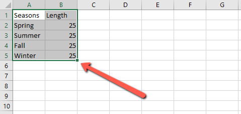
2
Highlight the spreadsheet data that will be contained in the chart.
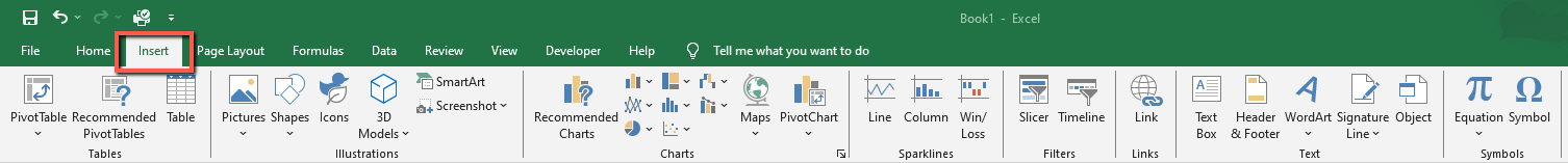
3
While the data is selected, left click on "Insert" in the top menu.
4
Select “Pie” and then click the pie chart of your choice.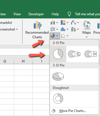
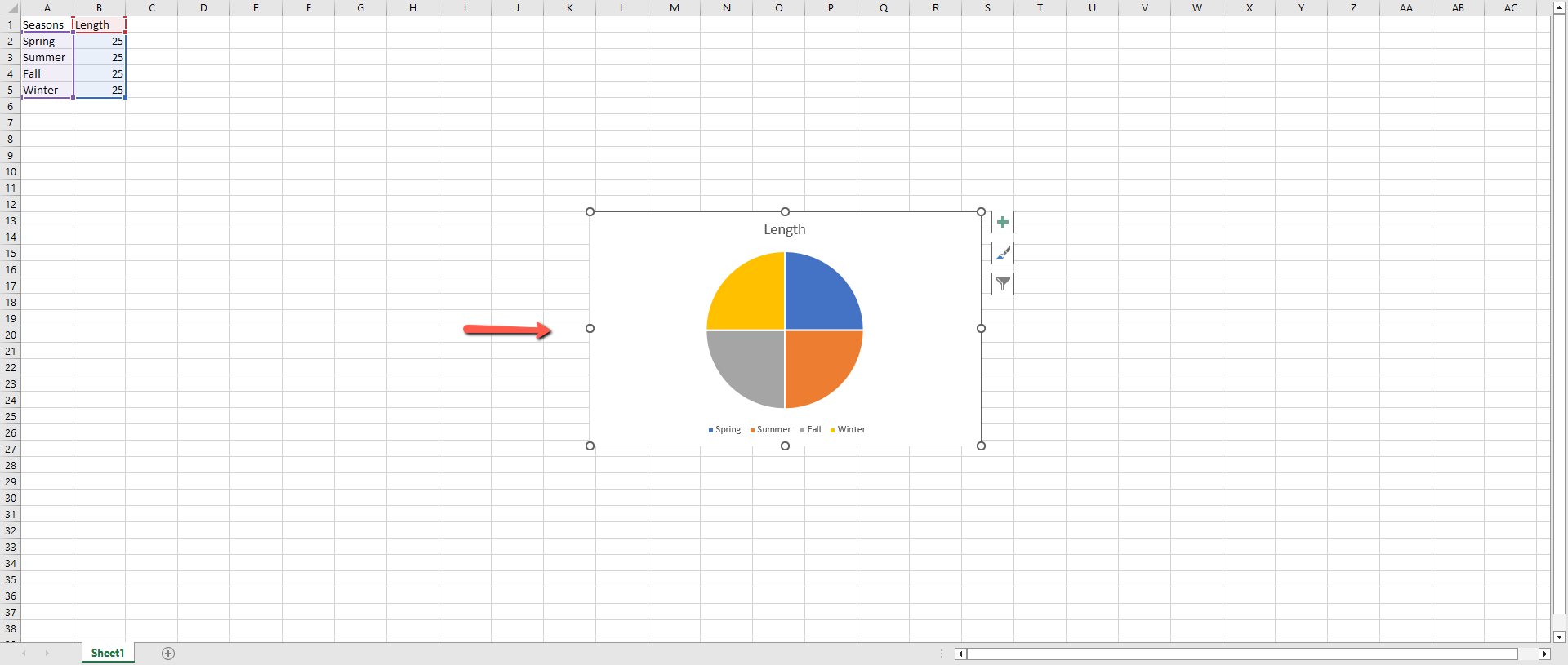
5
The pie chart should now be inserted into your spreadsheet somewhere near or in the center of the page.
Feel free to make any further edits to the chart or the data in the cells.
6
This task should be complete. Review the steps if you had any issues and try again. Submit questions or request for more guides in the questions section below.comments powered by Disqus
 Ask a question or provide an answer