


This guide is part of the Microsoft Excel 2010 series
1.
Add a print button to the tool bar in excel 2010
2. Create a bar graph in Excel 2010
3. How to add a background image to excel 2010
4. How to add a column to a spreadsheet in excel 2010
5. How to add a URL to Excel 2010
6. How to adjust the print layout in Excel 2010
7. How to auto fit column width in excel 2010
8. How to convert a column into a row in Excel 2010
9. How to convert excel 2010 to PDF
10. How to create a dashboard in Excel 2010
Make: Microsoft
Model / Product: Excel
Version: 2010
Objective / Info: Learn how to create a graph in Excel 2010.
Model / Product: Excel
Version: 2010
Objective / Info: Learn how to create a graph in Excel 2010.
1
Double click the icon on your desktop or start menu to open Excel.
2
Double click the "blank workbook" option.

3
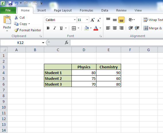
Populate the workbook with data you want to plot in a chart.
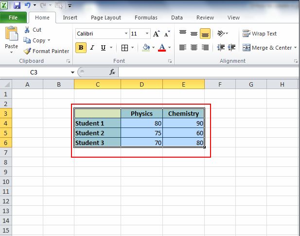
4
Select the data range along with the headings of each column. You can do this by left clicking the mouse button over the first row and column (C3 in this example) and keeping it pressed while dragging the mouse over the entire data range that you want to select.
Note :
You can also select the data by simply keeping the shift key pressed while clicking on first row and column and the last row and column you wish to select.
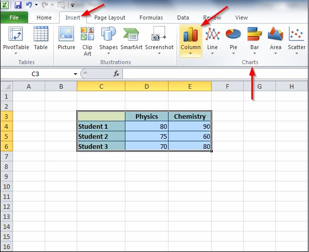
5
Choose the insert tab to select the chart type under the charts group.
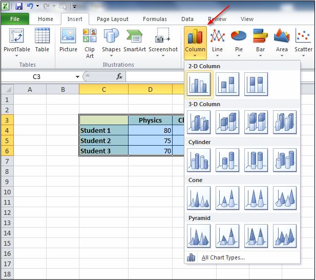
6
Select the subtype of the chart listed under the chart type you have chosen.
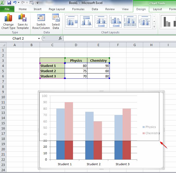
7
To re-size the graph/chart, drag its corners and adjust as per your preference.
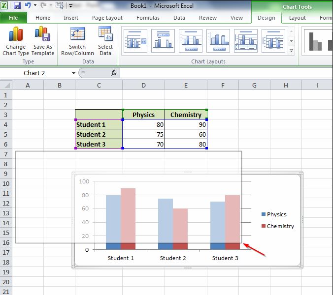
8
Drag the graph/chart from its white background to move it at your desired location on the workbook.
9
This task should be complete. Review the steps if you had any issues and try again.Submit questions or request for more guides in the questions section below.comments powered by Disqus
 Ask a question or provide an answer