how to create a pivot table in excel 2010

How to Create a Pivot Table in Excel 2010

Posted By tech

This guide is part of the Microsoft Excel 2010 series

1. Add a print button to the tool bar in excel 2010
2. Create a bar graph in Excel 2010
3. How to add a background image to excel 2010
4. How to add a column to a spreadsheet in excel 2010
5. How to add a URL to Excel 2010
6. How to adjust the print layout in Excel 2010
7. How to auto fit column width in excel 2010
8. How to convert a column into a row in Excel 2010
9. How to convert excel 2010 to PDF
10. How to create a dashboard in Excel 2010

Make: Microsoft

Model / Product: Excel

Version: 2010

Objective / Info: Learn To Create A Pivot Table In Excel 2010.

Launch Excel by clicking on the desktop icon.

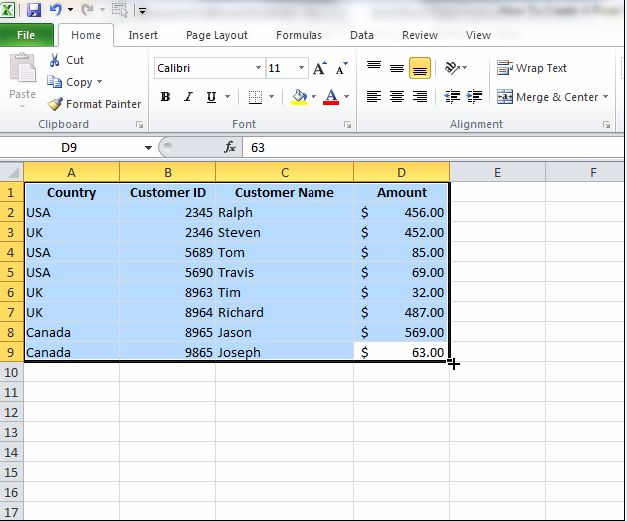
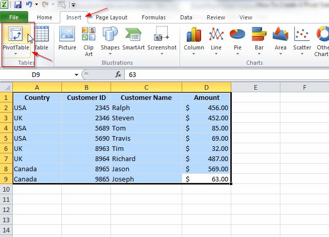
First of all, fill the Excel Worksheet with the relevant data. Now, select the entire data range you wish to create pivot table for.

Go to the ‘Insert’ tab and click the ‘Pivot Table’ icon to insert the Pivot Table.

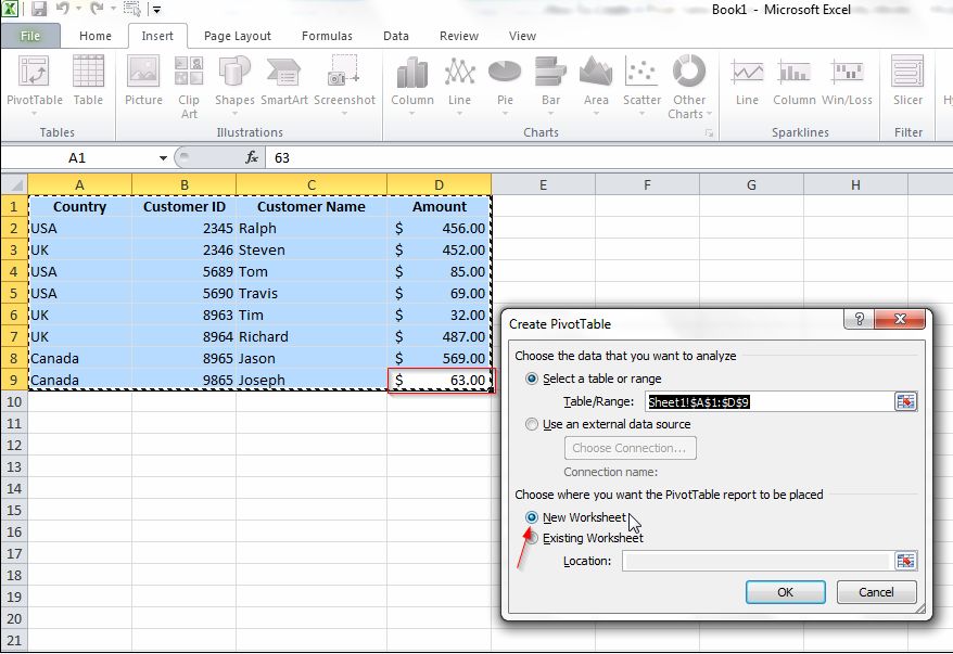
Select the targeted cell you wish the Pivot Table to be inserted in. For beginners, select ‘New Worksheet’ option to create the new worksheet with the Pivot Table.

Note : You can carry out various operations on this table for enhanced presentation and visualization of data.

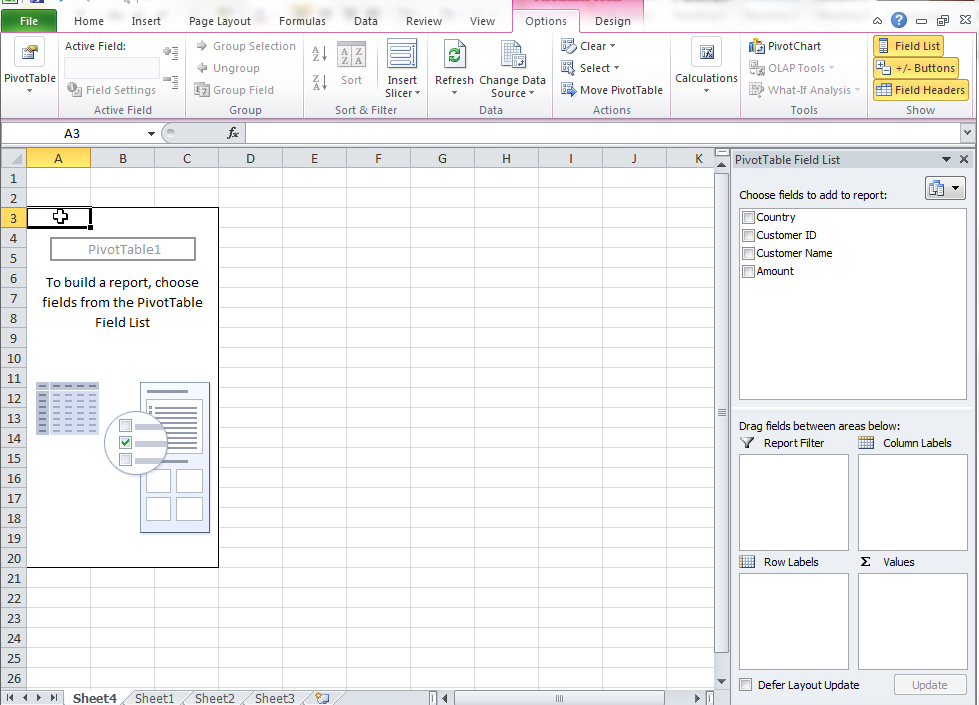
The new worksheet will open. On the right, you can see the Pivot Table Panel containing useful options for working with the table.

This task should be complete. Review the steps if you had any issues and try again.Submit questions or request for more guides in the questions section below.