


This guide is part of the Microsoft Excel 2010 series
1.
Add a print button to the tool bar in excel 2010
2. Create a bar graph in Excel 2010
3. How to add a background image to excel 2010
4. How to add a column to a spreadsheet in excel 2010
5. How to add a URL to Excel 2010
6. How to adjust the print layout in Excel 2010
7. How to auto fit column width in excel 2010
8. How to convert a column into a row in Excel 2010
9. How to convert excel 2010 to PDF
10. How to create a dashboard in Excel 2010
Make: Microsoft
Model / Product: Excel
Version: 2010
Objective / Info: Learn to freeze a column in an Excel spreadsheet.
Model / Product: Excel
Version: 2010
Objective / Info: Learn to freeze a column in an Excel spreadsheet.
1
Open Excel by double left clicking the icon on the desktop or start menu or open the document that you want to work on.
2
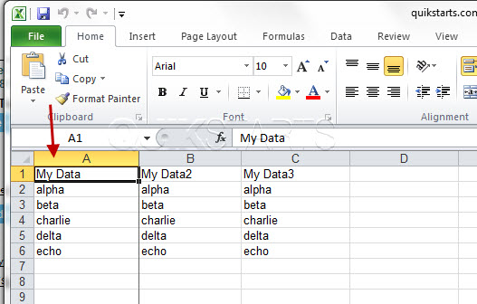
Click the column that you want to freeze. In this example we are going to freeze column A.
3
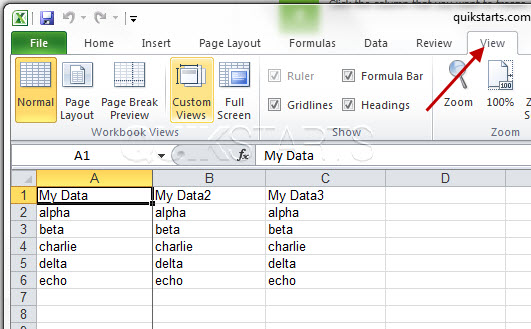
Click the "View" button on the menu.
4
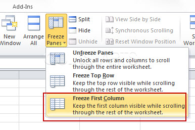
Click the "Freeze Panes" button on the menu bar.
Note :
Column A should now be frozen.
5
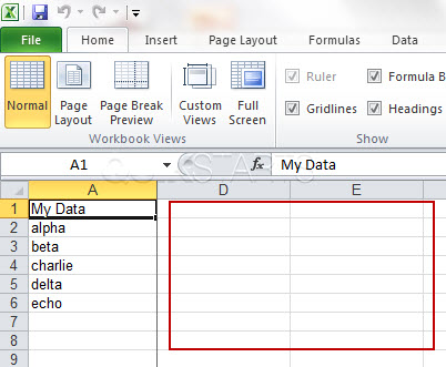
To test that you have successfully frozen the column, slide the horizontal scroll bar at the bottom of the page to the right and only columns B or greater should move, column A should not move.
6
This task should be complete. Review the steps if you had any issues and try again.Submit questions or request for more guides in the questions section below.comments powered by Disqus
 Ask a question or provide an answer